41 stories
·
0 followers

Competing for the JOB with a Triplestore

1 Share

JOB performance

This is a post about Datalevin, an open-source database system that I have been building since 2020. Although JOB here is really an acronym for Join Order Benchmark, a benchmark for complex database queries, I intend to build up Datalevin to compete for the same kind of jobs usually held by a RDBMS. I hope this title is received well and not seen as just a pun :-). This post describes my journey in making Datalevin competitive in the JOB benchmark, where it outperformed PostgreSQL by a small margin.

Datalevin is a triplestore, which means it stores data in units of three elements known as triples. Specifically, the three elements are entity (E), attribute (A) and value (V). For example, to store a piece of information: a person is named "John Smith", E would be the entity id number of this person, A would be an attribute named :person/name , and V would be "John Smith", the attribute value of the entity.

Unlike what the Wikipedia page of triplestore seems to suggest, a triplestore is not necessarily about Semantic Web use cases. Datalevin is a general purpose database system that follows an approach pioneered by Datomic, and uses its flavor of Datalog as the query language.

Why Datalog?

The flavor of Datalog used in Datalevin can be considered a modern alternative to SQL.

There have been many articles discussing the limitations of SQL as a database query language, such as Against SQL and We can do better than SQL, and I am sympathetic towards those views and recommend readers to look into them.

One point I would like to add, from a point of view of human computer interaction, is related to the historical context of SQL [1]. As one of those ALL CAP languages (e.g. COBOL), SQL was from an era when enthusiastic computer scientists believed that structured English could be a good human interface to computers. The rationale was that business people could be taught to use such languages to communicate with computers. We all know how that turned out: business people are allergic to any kind of formal languages, i.e. code, so these languages still end up as tools for programmers only. However, structured English makes for poor programming languages, because it is difficult to parse, compose or extend. SQL is the most stubborn left-over from those ill-considered experiments, perhaps due to the fact that data often last longer than programs.

Datalog used in Datalevin does not have such historical baggage. Let us look at an example:

;; query about persons who are adult males, whose name ends with Smith

[:find ?name
 :where
 [?person :person/age ?age]
 [?person :person/name ?name]
 [(like ?name "%Smith")]
 [(<= 18 ?age)]]

Similar to SQL's SELECT and WHERE, this flavor of Datalog has explicit :find and :where sections, so it is easier to grok than the original Datalog syntax from Prolog, which read like math expressions. Unlike SQL though, this query language is represented as a data structure in EDN format, which is amicable to programmatic manipulation, just like JSON.

Each where clause is delimited by a pair of [ ]. All the where clauses are AND'ed together, i.e. they all must evaluate to be true for the query to return non-empty results. There are two types of where clauses in this query: triple patterns and predicates.

Just like a triple, a triple pattern consists of Entity (E), Attribute (A) and Value (V), in that order. Any of the three elements could be a variable, which is a user defined symbol starting with a ?. For example, triple pattern [?person :person/age 18] says that there are entities that we name with a variable ?person, and they have an attribute :person/age with the value 18. Triple patterns must match with the data, so that variables can be bound with values from the database. For this pattern, ?person would be bound with entity IDs of all persons aged 18 in the database.

Predicates are boolean functions, and they are enclosed in a pair of ( ). The first element inside the parentheses is the function name, e.g. like, <=, and so on, and the rest are the function arguments. All the predicates must evaluate to be true for the query to return non-empty results.

That's it, the syntax of Datalevin's Datalog. There is neither complex syntactic rules, nor hundreds of reserved words.

More importantly, Datalog is very high level and truly declarative. It does not expose low level technical details of database operations to the users, nor requires the users to speak database jargons or be a relational algebra expert to use the language well. For example, the user is not required to understand the concept of joins, let alone the many different types of joins: inner, left, right, full, self joins, etc.

Joins are implicit in Datalog and are completely oblivious for the users. All users need to focus on are the logic relationships in their data, the rest is left for the database system to figure out. Datalog greatly simplifies the writing of complex queries. This is perhaps the main strength of this query language. My experience in onboarding new users has been that it normally took people less than half an hour to become a competent Datalog query writer.

Regardless the language level differences, Datalog in Datalevin is still backed up by a computational substrate based on relational algebra. It just treats relational algebra as underlying implementation details that users should not be concerned with.

Why a triple store?

When people talk about relational databases, they often assume it's a row store or a column store, as if relational algebra has something to do with how a table is stored. But, it doesn't. As a mathematical theory, relational algebra does not specify how a relation should be stored in computers. Therefore, in addition to storing a relation as rows or columns, storing it as triples are equally sound, if not better.

Example Data

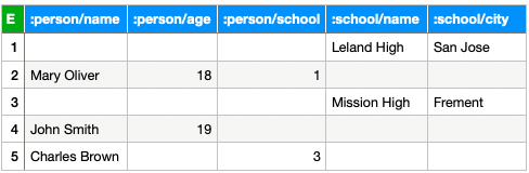
For example, for the data set above, a row store would store them as two tables.

Person Table School Table

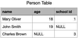
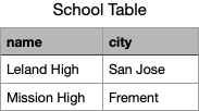
Storing a table as triples means storing the table as a list of table cells, i.e. as a list of the smallest identifiable units of the table.

Triples in EAV order

Storing table cells as rows or columns are just two concrete ways of bundling the table cells together for efficiency purpose, so that column identifiers or row identifier would not need to be repeated. That is to say, they are optimizations. So, the question is, are these "premature optimizations"?

I argue that they are. One problem with fixating the storage to either a row or a column format, is that it impedes querying the data later on. Specifically, it makes the work of query optimizer unnecessarily hard.

Essentially, both row and column storage are place oriented: table cells are identified by positions, rather than by explicit identifiers. One consequence is that missing data cells still have to be represented positionally, i.e. they need to take up places. RDBMS normally store these as special null values. This is what complicates the collection of statistics of table cells, which a query optimizer demands: it needs to know how many non-null data points it is dealing with under all kinds of conditions. The place based storage does not have a cheap way of providing this information, because any position could hold a null value, or not.

To work around this problem, RDBMS resorts to expensive and complicated processes to collect various approximations of exact data counts, e.g. histograms. Still, the lack of direct information often forces the optimizer to make unrealistically simplistic statistical assumptions about data distribution, e.g. independence, uniformity, and so on. This so called "cardinality estimation" problem is such a notoriously hard topic in database research that it is sometimes called "Achilles Heel" of database query processing [2].

In a triplestore, each table cell is identified explicitly by both row and column, e.g. E is the row, A is the column, and V is the value. A triple alone has complete information about a piece of data. Hence, a triple is called a datom (data atom) in this flavor of Datalog. Some simplifications naturally arise in such a triplestore.

In a triplestore, a missing table cell is simply missing from the storage: null is not stored, and absence means null. To remove a piece of data, one actually removes it from the storage, instead of setting some values to null. This is a critical simplification that enables easy and accurate counting of non-null data in the database.

Another simplification is that the entire database is essentially just one big table. E, A and V are all globally scoped. In Datalevin, E is represented as a 64 bit integer, and A a 32 bit integer. Database schema specifies only information about each attribute, e.g. its id, data type, uniqueness, and so on.

;; Datalevin schema for the example data above

{:person/name   {:db/aid 1 :db/valueType :db.type/string}
 :person/age    {:db/aid 2 :db/valueType :db.type/long}
 :person/school {:db/aid 3 :db/valueType :db.type/ref}
 :school/name   {:db/aid 4 :db/valueType :db.type/string}
 :school/city   {:db/aid 5 :db/valueType :db.type/string}}

Information about individual tables are no longer necessary. Name spaced attribute names still allow grouping of attributes, e.g. :person/name, person/age are attributes of person entity, but this is just a convention, not a physically separated table. Tables dedicated to joins also disappear, as they are simply handled by attributes with entity id as values (i.e. of reference data type: :db.type/ref).

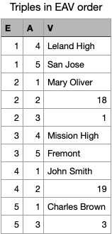
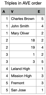
The atomic nature of a datom allows maximum flexibility, as these datoms can be arranged in ways that facilitate querying them. For example, if datoms are ordered by E first, then A, then V, one essentially gets a row major storage that has the similar properties of a row store. If datoms are ordered by A first, one gets a column major storage that has the same advantage of a column store. Tripestores often store data in both orderings, so that essentially all data are indexed by default. Not having to manage indices can save some headache.

Triples in AVE order

Obviously, the storage of triplestores is redundant, as row identifiers and column identifiers are repeated. If storing both row major and column major data ordering, even more storage spaces are taken. More data means higher I/O demand, and slower querying may be resulted. This is perhaps the main challenge that has prevented the widespread use of triplestores.

I argue that this data storage redundancy problem is easier to mitigate than the hard problem of cardinality estimation resulted from bundling table cells as rows or columns. For example, prefix compression could be used to minimize the repetition. Datalevin utilizes this strategy by storing data in a two level nesting schema: AV is nested underneath E in EAV ordering, and E underneath AV in AVE ordering. Obviously, three level nesting can further reduce data redundancy.

Critically, with unbundled table cells in triplestores, the problem of cardinalty estimation can be solved with straightforward counting or sampling. I argue that this advantage is perhaps a good reason to use a triplestore. As a demonstration, Datalevin employed this simple strategy of counting and sampling to achieve better performance than PostgreSQL in JOB benchmark.

Join Order Benchmark (JOB)

This benchmark aims to test a database query optimizer's capacity to handle complex queries that involve many joins [3]. Based on Internet Movie Database, 113 analytical SQL queries were developed to have between 3 and 16 joins, with an average of 8 joins per query. These SQL queries were translated into the equivalent Datalevin queries, which were verified to produce exactly the same results as corresponding SQL ones.

The tests were conducted on a MacBook Pro Nov 2023, Apple M3 Pro chip, 6 performance cores and 6 efficiency cores, 36GB memory, and 1TB SSD disk.

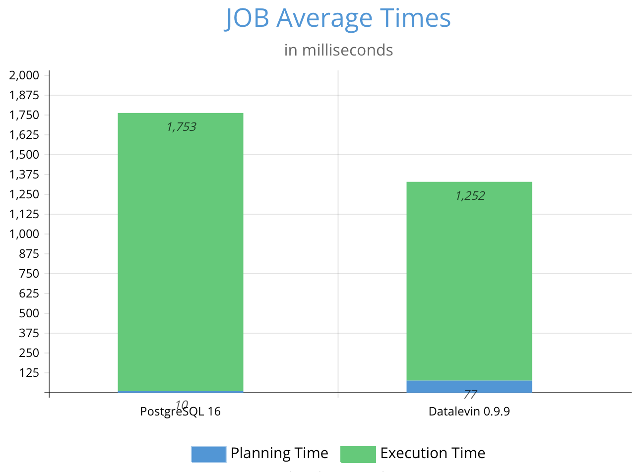
On average, Datalevin is about 1.3 times faster than PostgreSQL 16 in this benchmark. More details can be found here.

Analysis

Given that Datalevin is written in Clojure — a functional programming language on JVM, not widely known for speed, and PostgreSQL is written in highly optimized C code, it's clear that the query optimizer of Datalevin generates better execution plans than that of PostgreSQL on average.

As I will show with an example, Datalevin's better plan is mainly achieved by having more accurate estimate of result sizes at each execution step, corroborating with the point argued above regarding the superiority of triplestores.

Query 20a of JOB is what PostgreSQL did the worst compared with Datalevin. It took PostgreSQL over a minute to execute its plan whereas Datalevin took about a second. Let us look at the SQL query first.

-- query 20a

SELECT MIN(t.title) AS complete_downey_ironman_movie
FROM complete_cast AS cc,
     comp_cast_type AS cct1,
     comp_cast_type AS cct2,
     char_name AS chn,
     cast_info AS ci,
     keyword AS k,
     kind_type AS kt,
     movie_keyword AS mk,
     name AS n,
     title AS t
WHERE cct1.kind = 'cast'
  AND cct2.kind LIKE '%complete%'
  AND chn.name NOT LIKE '%Sherlock%'
  AND (chn.name LIKE '%Tony%Stark%'
       OR chn.name LIKE '%Iron%Man%')
  AND k.keyword IN ('superhero',
                    'sequel',
                    'second-part',
                    'marvel-comics',
                    'based-on-comic',
                    'tv-special',
                    'fight',
                    'violence')
  AND kt.kind = 'movie'
  AND t.production_year > 1950
  AND kt.id = t.kind_id
  AND t.id = mk.movie_id
  AND t.id = ci.movie_id
  AND t.id = cc.movie_id
  AND mk.movie_id = ci.movie_id
  AND mk.movie_id = cc.movie_id
  AND ci.movie_id = cc.movie_id
  AND chn.id = ci.person_role_id
  AND n.id = ci.person_id
  AND k.id = mk.keyword_id
  AND cct1.id = cc.subject_id
  AND cct2.id = cc.status_id;

The PostgreSQL EXPLAIN ANALYZE output for this query:

                                                                                          QUERY PLAN
-----------------------------------------------------------------------------------------------------------------------------------------------------------------------------------------------
 Nested Loop  (cost=21.78..2474.54 rows=1 width=17) (actual time=17052.871..72628.822 rows=33 loops=1)
   ->  Nested Loop  (cost=21.35..2474.09 rows=1 width=21) (actual time=17052.352..72626.880 rows=33 loops=1)
         ->  Nested Loop  (cost=20.93..2473.63 rows=1 width=25) (actual time=17042.110..72584.290 rows=1314 loops=1)
               ->  Nested Loop  (cost=20.50..2473.17 rows=1 width=29) (actual time=1.352..35903.879 rows=87986607 loops=1)
                     Join Filter: (ci.movie_id = t.id)
                     ->  Nested Loop  (cost=20.06..2471.42 rows=1 width=33) (actual time=1.124..3346.138 rows=978322 loops=1)
                           ->  Nested Loop  (cost=19.63..2469.68 rows=1 width=25) (actual time=0.703..2394.487 rows=28583 loops=1)
                                 ->  Nested Loop  (cost=19.48..2469.50 rows=1 width=29) (actual time=0.688..2362.288 rows=73560 loops=1)
                                       ->  Nested Loop  (cost=19.05..2467.72 rows=1 width=4) (actual time=0.444..41.257 rows=85941 loops=1)
                                             ->  Hash Join  (cost=18.89..2462.46 rows=190 width=8) (actual time=0.416..22.960 rows=135086 loops=1)
                                                   Hash Cond: (cc.status_id = cct2.id)
                                                   ->  Seq Scan on complete_cast cc  (cost=0.00..2086.86 rows=135086 width=12) (actual time=0.365..6.616 rows=135086 loops=1)
                                                   ->  Hash  (cost=18.88..18.88 rows=1 width=4) (actual time=0.035..0.035 rows=2 loops=1)
                                                         Buckets: 1024  Batches: 1  Memory Usage: 9kB
                                                         ->  Seq Scan on comp_cast_type cct2  (cost=0.00..18.88 rows=1 width=4) (actual time=0.027..0.028 rows=2 loops=1)
                                                               Filter: ((kind)::text ~~ '%complete%'::text)
                                                               Rows Removed by Filter: 2
                                             ->  Memoize  (cost=0.16..0.18 rows=1 width=4) (actual time=0.000..0.000 rows=1 loops=135086)
                                                   Cache Key: cc.subject_id
                                                   Cache Mode: logical
                                                   Hits: 135084  Misses: 2  Evictions: 0  Overflows: 0  Memory Usage: 1kB
                                                   ->  Index Scan using comp_cast_type_pkey on comp_cast_type cct1  (cost=0.15..0.17 rows=1 width=4) (actual time=0.119..0.119 rows=0 loops=2)
                                                         Index Cond: (id = cc.subject_id)
                                                         Filter: ((kind)::text = 'cast'::text)
                                                         Rows Removed by Filter: 0
                                       ->  Index Scan using title_pkey on title t  (cost=0.43..1.78 rows=1 width=25) (actual time=0.027..0.027 rows=1 loops=85941)
                                             Index Cond: (id = cc.movie_id)
                                             Filter: (production_year > 1950)
                                             Rows Removed by Filter: 0
                                 ->  Index Scan using kind_type_pkey on kind_type kt  (cost=0.15..0.17 rows=1 width=4) (actual time=0.000..0.000 rows=0 loops=73560)
                                       Index Cond: (id = t.kind_id)
                                       Filter: ((kind)::text = 'movie'::text)
                                       Rows Removed by Filter: 1
                           ->  Index Scan using movie_id_movie_keyword on movie_keyword mk  (cost=0.43..1.29 rows=46 width=8) (actual time=0.024..0.031 rows=34 loops=28583)
                                 Index Cond: (movie_id = t.id)
                     ->  Index Scan using movie_id_cast_info on cast_info ci  (cost=0.44..1.31 rows=35 width=12) (actual time=0.001..0.028 rows=90 loops=978322)
                           Index Cond: (movie_id = mk.movie_id)
               ->  Index Scan using char_name_pkey on char_name chn  (cost=0.43..0.46 rows=1 width=4) (actual time=0.000..0.000 rows=0 loops=87986607)
                     Index Cond: (id = ci.person_role_id)
                     Filter: ((name !~~ '%Sherlock%'::text) AND ((name ~~ '%Tony%Stark%'::text) OR (name ~~ '%Iron%Man%'::text)))
                     Rows Removed by Filter: 0
         ->  Index Scan using keyword_pkey on keyword k  (cost=0.42..0.45 rows=1 width=4) (actual time=0.032..0.032 rows=0 loops=1314)
               Index Cond: (id = mk.keyword_id)
               Filter: (keyword = ANY ('{superhero,sequel,second-part,marvel-comics,based-on-comic,tv-special,fight,violence}'::text[]))
               Rows Removed by Filter: 1
   ->  Index Only Scan using name_pkey on name n  (cost=0.43..0.45 rows=1 width=4) (actual time=0.059..0.059 rows=1 loops=33)
         Index Cond: (id = ci.person_id)
         Heap Fetches: 0
 Planning Time: 28.727 ms
 Execution Time: 72629.051 ms
(50 rows)

As can be seen, the catastrophic running time is mainly due to vastly underestimated result join sizes, leading to sub-optimal join order. For instance, the planner estimated that the hash join of complete_cast and comp_cast_type would produce 190 rows but actually got 135086 rows. Similar under-estimation is persisted and its effect accumulated, eventually reaching a staggering 1 vs. 87986607 discrepancy with actual result size.

These underestimations are due to the strong statistical assumptions its estimator makes: value uniformity and column independence. However, the actual value distribution is highly skewed and the columns are highly correlated with one another, as it is often the case in real world datasets. I would like to point out that this problem is not unique to PostgreSQL, but in fact common in all row based RDBMS [3]. These strong assumptions are necessary because more direct information is not available in row stores.

Datalevin does not rely on such strong statistical assumptions to estimate join result size. Instead, it simply counts or samples to obtain the base selectivity ratios. Then, for each pair of base relations, it actually executes the joins using the samples, and thus obtains the pair-wise join selectivity ratios. These rations are simply used in estimation of join sizes in later joins. The only assumption it makes is that the base selectivity ratios are similar to those of later joins. If the samples are representative, this assumption would not be too off base.

For query 20a, the corresponding Datalog query is the following:

            ;; query 20a

            [:find (min ?t.title)
             :where
             [?cct1 :comp-cast-type/kind "cast"]
             [?cct2 :comp-cast-type/kind ?cct2.kind]
             [(like ?cct2.kind "%complete%")]
             [?chn :char-name/name ?chn.name]
             [(not-like ?chn.name "%Sherlock%")]
             [(or (like ?chn.name "%Tony%Stark%") (like ?chn.name "%Iron%Man%"))]
             [?k :keyword/keyword ?k.keyword]
             [(in ?k.keyword ["superhero", "sequel", "second-part",
                              "marvel-comics", "based-on-comic",
                              "tv-special", "fight", "violence"])]
             [?kt :kind-type/kind "movie"]
             [?t :title/production-year ?t.production-year]
             [(< 1950 ?t.production-year)]
             [?t :title/kind ?kt]
             [?mk :movie-keyword/movie ?t]
             [?ci :cast-info/movie ?t]
             [?cc :complete-cast/movie ?t]
             [?ci :cast-info/person-role ?chn]
             [?ci :cast-info/person ?n]
             [?mk :movie-keyword/keyword ?k]
             [?cc :complete-cast/subject ?cct1]
             [?cc :complete-cast/status ?cct2]
             [?t :title/title ?t.title]]

The :plan portion of the explain output is the following:

  [[{:steps       ["Initialize [?k ?k.keyword] by range [[[:closed \"based-on-comic\"] [:closed \"based-on-comic\"]] [[:closed \"fight\"] [:closed \"fight\"]] [[:closed \"marvel-comics\"] [:closed \"marvel-comics\"]] [[:closed \"second-part\"] [:closed \"second-part\"]] [[:closed \"sequel\"] [:closed \"sequel\"]] [[:closed \"superhero\"] [:closed \"superhero\"]] [[:closed \"tv-special\"] [:closed \"tv-special\"]] [[:closed \"violence\"] [:closed \"violence\"]]] on :keyword/keyword."],
     :cost        17,
     :size        8,
     :actual-size 8}
    {:steps       ["Merge ?mk by reverse reference of :movie-keyword/keyword."
                   "Merge [?t] by scanning [:movie-keyword/movie]."],
     :cost        41,
     :size        35549,
     :actual-size 35548}
    {:steps       ["Merge ?cc by equal values of :complete-cast/movie."
                   "Merge [?cct2 ?cct1] by scanning [:complete-cast/status :complete-cast/subject]."],
     :cost        147569,
     :size        11909,
     :actual-size 12810}
    {:steps       ["Merge ?ci by equal values of :cast-info/movie."
                   "Merge [?chn ?n] by scanning [:cast-info/person-role :cast-info/person]."],
     :cost        196991,
     :size        472311,
     :actual-size 476091}
    {:steps       ["Merge [?chn.name] by scanning [:char-name/name]."],
     :cost        2180697,
     :size        472,
     :actual-size 33}
    {:steps       ["Merge [?t.title ?kt ?t.production-year] by scanning [:title/title :title/kind :title/production-year]."],
     :cost        2184661,
     :size        472,
     :actual-size 33}
    {:steps       ["Filter by predicates on [:comp-cast-type/kind]."],
     :cost        2186643,
     :size        472,
     :actual-size 33}
    {:steps       ["Filter by predicates on [:kind-type/kind]."],
     :cost        2188625,
     :size        472,
     :actual-size 33}
    {:steps       ["Merge [?cct2.kind] by scanning [:comp-cast-type/kind]."],
     :cost        2190607,
     :size        472,
     :actual-size 33}]]

As can be seen, the estimated join sizes are close to the actual sizes. Particularly for the initial steps, the estimations are almost exact. For data sizes that smaller than a user configured threshold, actual counting of the data is performed, while sampling was performed for larger data sizes. Both are performed under query specific conditions.

Compared with the tree shape of the PostgreSQL's plan, the plan in Datalevin is linear, because we only consider left-deep join tree. We join one base relation at a time in order to take advantage of the accurate counting and sampling of base relations.

Counting and sampling under query conditions are straightforward in Datalevin, thanks to the nested triple storage. Applicable value predicates are translated into range queries in AVE ordering of triples. When both A and V is known, obtaining the count is a constant time operation. When V is a range, the count is just the sum of the counts in range; The only missing information is total count of A, which is easily maintained during transaction.

More details of the Datalevin query planner and execution engine can be found here.

Summary

With Datalevin, I have demonstrated that a triplestore has some unique advantages compared with row or column based databases. It helps with solving the difficult problem of cardinality estimation, while its shortcomings can be easily mitigated by nested storage of triples. Paired with a Datalog query language, it makes a promising choice as a modern alternative to SQL RDBMS, as it is much more ergonomic.

References

[1] Chamberlin, D. and Boyce, R.. "SEQUEL: A Structured English Query Language", Proc. ACM SIGFIDET Workshop on Data Description Access and Control. 1974.

[2] Leis, V., et al. "Cardinality Estimation Done Right: Index-Based Join Sampling." Cidr. 2017.

[3] Leis, V., et al. "How good are query optimizers, really?." VLDB Endowment. 2015.

Read the whole story
yqrashawn
34 days ago
reply
Share this story
Delete

Nyxt browser: keyboard.org

1 Share

Abstract

On why the keyboard is likely to remain the leading input device for knowledge workers, how keyboard design impacts ergonomics, and the consequences that keyboard firmware has on the design of advanced shell programs (those that expose the OS to end users).

Input devices

Unlike typical users who interact with information systems in the way they were meant to be used, knowledge workers constantly craft them as to attain optimized workflows. Notice that the process is continuous, since the tasks they use their systems for are a moving target.

Keyboards have been the primary input device for these systems. As their adoption became widespread, more intuitive interfaces have been devised, namely voice interfaces. While intuitive, they are unlikely to replace the keyboard for knowledge workers altogether. Besides being physiologically challenging to use one's voice over long periods of time, it also accounts to a single serial channel, while the keyboard provides ten channels that can be almost regarded as parallel.1

Voice input may be used to enter a first draft of textual information to be subsequently edited with the keyboard. Note that error correction by voice is inefficient. More broadly, from all of the instructions that users send to these systems, few fall in the category where voice input excels.

Some have gone to great lengths to perform complex tasks such as moving the cursor, selecting pieces of text or managing windows by voice.2 It should be noted that the motivation for such endeavors are RSI (repetitive strain injury) and sheer curiosity. The claim that it is pinnacle of efficiency has no support, given the design of today's systems.

The popularity of voice user interfaces in on the rise and it seems reasonable to anticipate that it will become the preferred input method for typical end users. For knowledge workers, however, it may be a mere complementary input device, similar to the role played by pointing devices such as mice, trackballs or touchpads.

Keyboard design and ergonomics

For decades, researchers have been conducting experiments that measure arm strain and proposing alternative keyboard designs such as split keyboards, whose patents appear as early as 1915 by F. Heidner.3 4 The next paragraphs detail how the design of modern split keyboards improve ergonomics, namely by avoiding ulnar deviation, wrist extension and arm pronation.

Take the line that connects the elbow to the wrist, and another connecting the middle of the wrist to the tip of the middle finger. Ulnar deviation is observed when these two lines aren't parallel. Split keyboards avoid it by enabling typing at shoulder width.

Keyboard feet (below the Fn-keys row) cause wrist extension. Since this is undesirable from an ergonomics perspective, providing the user a better overview of the keys is a plausible explanation for its existence. But all knowledge workers are touch typists, thus making them useless. From an ergonomics standpoint, the keyboard should lie flat or at a negative angle (for instance, by placing feet where the wrists rest).

Arm pronation results from laying the palm of our hands down on a table. This isn't the most natural position and keyboard "tenting" mitigates it. The "tenting" is achieved by placing feet on the inner side of each keyboard half.

While fingers move along straight lines, the ANSI/ISO keyboard features row stagger (the A and Z keys are indented with respect to the Q key). Unfortunately, as the mechanical typewriters predate modern keyboards, they have inherited this poor design that prevented the mechanical jamming of keys. Column stagger, on the other hand, makes perfect sense since it accounts for the different lengths of the fingers. The standard keyboard makes little use of the thumbs. Given their strength, it is unfortunate that the space key is so wide since the thumbs could cover more keys.

As a side node on the topic of ergonomics, it is often argued that reaching out for the the mouse must be avoided at all costs. It is inefficient to do it several times per minute (e.g. to adjust the cursor), but that doesn't mean that ditching pointing devices altogether is wise. The golden rule in ergonomics says that sustained periods in any position are to be avoided.

The Sofle keyboard5 in an example of a design that takes all of these considerations into account.

Keyboard Firmware and QMK

QMK6 is a project centered around developing firmware for computer input devices. Find a very superficial overview of some of its features below.

Layers. Think of Fn key, found on laptops, as a way to assign more functions to the same set of physical keys. In QMK, a layer is a 2D array whose dimensions are dictated by the physical keys of the keyboard and the values are keycodes. A keymap is a list of these layers (a 3D array), i.e. a stack of them and only a single layer is active at any given time. If you are familiar with the Fn lock button, then the concept of momentary and latching layer keys is also clear.

Mod taps. On tap they behave like regular keys, while on hold they act like a modifier keys. The consequences are far reaching. There is no longer the need to assign a key to act exclusively as a modifier key. A typical configuration, known as home row mods7, assigns the home row keys to mod taps symmetrically. For instance (on QWERTY), holding F or J triggers Shift, holding D or K triggers Ctrl, holding S or L triggers Alt and A or ; triggers Super. The common 4 modifiers keys map perfectly to the 4 fingers and the mirror symmetry offloads some of the strain. For example, to produce Ctrl+f both hands should be used: holding K to produce Ctrl with the right hand, and tapping F with the left hand.

Tap dance. Send a different keycode depending on how many times a key is tapped.

Combos. Press several keys together to produce a particular action. Example, press Q and W together and trigger Esc.

Mouse emulation. Control the pointer with the keyboard. It isn't as accurate as other pointing devices but it avoids reaching out for one for simple tasks.

In short, this non-exhaustive set of features enables squeezing the number of required physical keys and thus keeping the fingers closer to the home row position. There is a vibrant community doing intense experimentation that culminates in systems such as Miryoku.8 9

For those who frequently use the laptop's keyboard or don't have a keyboard running QMK, it is possible to get a taste of its set of features thanks to Kmonad10. Find below how a basic keymap that implements home row mods and a navigation layer would look like in a Kmonad configuration file.

(defcfg
  input   (device-file "/dev/input/by-path/platform-i8042-serio-0-event-kbd")
  output  (uinput-sink "KMonad: Dell XPS 9350 (ISO keyboard)")
)

(defalias
  ;; Home row mods
  ;; "A" key on tap, Super key on hold
  *a (tap-hold-next-release 175 a meta)

  ;; "S" key on tap, Alt key on hold
  *s (tap-hold-next-release 175 s lalt)

  ;; "D" key on tap, Ctrl key on hold
  *d (tap-hold-next-release 175 d lctl)

  ;; "F" key on tap, Shift key on hold
  *f (tap-hold-next-release 175 f lsft)

  ;; Mirror modifiers keys on the right hand side
  *j (tap-hold-next-release 175 j lsft)
  *k (tap-hold-next-release 175 k lctrl)
  *l (tap-hold-next-release 175 l lalt)
  *; (tap-hold-next-release 175 ; meta)

  ;; "H" key on tap, enter Navigation layer on hold
  *h (tap-hold-next-release 175 h (layer-toggle nav))
)

;; Declare the keymap of the original keyboard, the usual ISO laptop keyboard
;; (slightly differs from ANSI).
(defsrc
  esc     f1      f2      f3      f4      f5      f6      f7      f8      f9      f10     f11     f12     prnt    ins     del
  `       1       2       3       4       5       6       7       8       9       0       -       =       bspc
  tab     q       w       e       r       t       y       u       i       o       p       [       ]
  caps    a       s       d       f       g       h       j       k       l       ;       '       \       ret
  lsft    lsgt    z       x       c       v       b       n       m       ,       .       /       rsft
  lctl            lmeta   lalt    spc                             ralt    rctrl           left    up      down    rght

  home    pgup    pgdn    end
)

;; Defines the default layer. The CapsLock/Ctrl swap illustrates how easy it is to remap keys.
(deflayer default
  esc     f1      f2      f3      f4      f5      f6      f7      f8      f9      f10     f11     f12     prnt    ins    del
  `       1       2       3       4       5       6       7       8       9       0       -       =       bspc
  tab     q       w       e       r       t       y       u       i       o       p       [       ]
  lctrl   @*a     @*s     @*d     @*f     g       @*h     @*j     @*k     @*l     @*;     '       \       ret
  lsft    lsgt    z       x       c       v       b       n       m       ,       .       /       rsft
  caps            lmeta   lalt    spc                             ralt    rctrl           left    up      down    rght

  home    pgup    pgdn    end
)

;; Navigation layer
;; The "_" means that the keycode from the default layer is used.
(deflayer nav
  _       _       _       _       _       _       _       _       _       _       _       _       _       _       _      _
  _       _       _       _       _       _       _       _       _       _       _       _       _       _
  _       pgup    home    up      end     _       _       _       _       _       _       _       _
  _       pgdn    left    down    rght    _       _       lsft    lctrl   lalt    meta    _       _       _
  _       _       _       _       _       _       _       _       _       _       _       _       _
  _               _       _       _                               _       _               _       _       _       _

  _       _       _       _
)

In the sections above, the keyboard has been analyzed from the perspective of ergonomics and firmware. Note that while Kmonad gives a taste of the latter, it improves the former by a very small margin. Nonetheless, it can be an interesting bridge solution for those considering experimenting with these ideas.

Consequences for advanced programs

Software that does keyboard configuration on the OS-level (AutoHotKey, xmodmap, etc) becomes obsolete. Given the importance of the keyboard in human-machine interaction, it is desirable to keep the configuration saved on the device as to ensure that it behaves the same regardless of the system it communicates with.11

Many advanced programs go to great lengths as to lessen the quirks of keyboard design. Emacs and vi bind commands to keys that are easier to reach on standard keyboards at the cost of intuitiveness. For instance, the motivation for binding C-n/p/f/b to cursor movements is grounded, but loses its actuality as soon as pressing the arrows keys becomes just as easy. Among QMK users, it is common practice to have a layer dedicated to navigation keys which is activated by holding down a thumb key. This way, it is possible to eliminate the discomfort of reaching out for these keys and to prefer semantic keybindings over cryptic ones, i.e. PgDn (PgUp) is easier to learn than C-v (M-v).

These programs also frequently implement keyboard macros as a feature of their own, which is not very efficient since each program needs to re-invent the wheel. This can theoretically be solved by having a cross-platform library that would make it easy to implement such a feature. But it would still be subpar. Keyboard macros obviously belong to keyboard firmware, and QMK provides it. It may not yet be as advanced as Emacs' implementation, but it's a solid step in the right direction.

The same argument as above can be made with respect to repeat keys. Emacs implements the feature (repeat.el), and so does QMK. But the latter provides a single implementation and constant behaviour for arbitrary programs and operating systems. QMK also defines an alternative repeat key that performs the dual behaviour of the last pressed key. For instance, if the hit last key was Backspace, then the alternative repeat key would trigger Delete. The same applies to key-chord.el (which is covered by QMK's combos).

The downfall of modal editing as implemented in vi or Kakoune12. The problem with the approach is that, when using several of such programs, the user needs to remember or check the modality state for a fraction of second when cycling between them. Even if we take 3 programs and each of those features 2 modes of operation, then the state space size is 8. In short, this approach doesn't scale. The idea behind modality is certainly interesting but it can be attained in different ways.13 If modality is implemented exclusively on the level of keyboard firmware, then the aforementioned issue vanishes since keeping track of mode toggling when using a single keyboard is easier. It is also possible to achieve modality with a momentary or latching switch. I.e., a layer that serves the purpose of vi's normal mode can be enabled while holding a key, or when a key is pressed and released (then another key press is needed to return to the former layer).

Conclusion

It is not the user-space software's responsibility to account for the idiosyncrasies of poor keyboard design standards. It is urgent to bring modern keyboard design (both hardware and firmware) to the mainstream among knowledge workers. Keyboard firmware that enables user customization is paramount. Tweaking the keyboard's firmware must be as easy as binding a command to a key in Nyxt.

Advanced shell programs become smaller when their users use proper keyboards, which allows for the developers to focus on the project's key goals and tame its complexity. In Nyxt's concrete case, the implementation of the repeat-key command, cruise-control-mode, macro-edit-mode and modal keyschemes would become redundant when using the ideas shared in this article. While redundancy is a characteristic of robust systems, there's still an important dimension to take into account, namely that of health and ergonomics.

Did you enjoy this article? Register for our newsletter to receive the latest hacker news from the world of Lisp and browsers!

Read the whole story
yqrashawn
370 days ago
reply
Share this story
Delete

Clojure Deref (Oct 6, 2023)

1 Comment

Welcome to the Clojure Deref! This is a weekly link/news roundup for the Clojure ecosystem (feed: RSS). Thanks to Anton Fonarev for link aggregation.

From the core

Recently Java 21 was released (congrats!) and this has driven a lot of interest and experimentation with the new virtual threads feature. Virtual threads have the ability to park and resume a virtual thread (particularly one blocked on I/O) and this cooperates transparently with many blocking constructs in Java - I/O, sockets, java.util.concurrent.lock, etc. However, one thing it does not (yet) cooperate with is object monitors (synchronized) and thus doing a blocking call while holding a synchronized monitor prevents a virtual thread from parking (ie, "pins" the virtual thread). Note that synchronization itself is not inherently bad - normal use of synchronized to serialize reads and writes to fields is fine (as there is no blocking I/O that can pin a thread).

Several people doing new things with virtual threads have detected cases where user code is doing I/O blocking while Clojure is in a synchronization block, thus pinning threads. The two most important cases are lazy seqs and delay - both hold some suspended computation in a thunk and invoke the thunk under synchronization, thus allowing for the possibility of user I/O under a lock in the language level. As people have raised this as an issue, we have spent the last week taking a hard look at this area.

At a meta level, there are a bunch of options here and we have still not decided on our approach or timeframe. From a user level, it is possible to simply not do (or tolerate) I/O under delay or lazy seqs. Delay is a one-time thing, so it may not generally be an issue to pin a thread that is reading a config file as that is a one-time thing. Pulling I/O over a lazy seq is not uncommon and can definitely present this kind of issue, but there are a lot of other options - controlling via loop/recur, using transducers and sequence, etc. If you are experiencing this problem now, these are probably worth exploring.

We’ve spent a ton of time over the last week looking at the internals of LazySeq and options for avoiding synchronization. The general guidance from Java is to replace synchronized with ReentrantLock (which has virtual thread coordination), but this advice leaves out the inherent tradeoffs in that change. synchronized relies on object monitors which are built into every Java object at the JVM level, whereas ReentrantLocks are additional Java objects (which hold a reference to an internal Sync object). Clojure makes a lot of lazy seqs and allocating two objects (plus adding an additional field to LazySeq) for every lazy seq is a real cost in allocation, heap size, and GC. Additionally, while ReentrantLock seems to be a bit faster than synchronized in Java 21, LazySeq makes one reentrant call, and reentrant calls seems to be noticeably slower than synchronized. There are lots of options though. We think it’s relatively easy to make lazy seq walking faster, but a lot harder to keep realization costs under control (as making locks takes non-zero time). One interesting branch we have explored is making one lock per seq and passing it through the seq as we go - lots of tradeoffs in that.

Additionally, we continue to work on functional interface adapters and method thunks. With FI adapters, we continue to refine when implicit coercion and conversion occur and I think that draws asymptotically closer to completion. With method thunks, we have taken a bit of a detour to examine array class representation.

Generally, classes are represented by symbols that name the class, but this does not work for array classes as they cannot be represented as a valid symbol. The fallback right now is using a String that holds the internal class name, like ^"[Ljava.lang.String;" which I think we can all agree is no fun. Our plan going forward is to support a new array class syntax which is a symbol of the class with a * suffix. Imported classes can use their short name, so String* will represent a Java String[] (or a String…​ vararg). Multiple ** will represent multidimensional arrays. This will work with both classes and with primitives, so long* will be a synonym for the existing longs. Rich also wishes you to notice the C pointer punnery. :)

That was a bit of a diversion, but I think it is a big win to fix a long-time representational gap. It also helps create some new "columns" in the varargs decision matrix, which is not going to be addressed in 1.12, but I think we have teed up to work on immediately after.

Libraries and Tools

New releases and tools this week:

  • fulcro-troubleshooting v7 - A development-time library for Fulcro that helps to detect problems earlier and find and fix their root cause faster

  • minimalist-fulcro-template-backendless - A minimal template for browser-only Fulcro apps for learning

  • clojure-test 2.1.182 - A clojure.test-compatible version of the classic Expectations testing library

  • clerk 0.15.957 - Moldable Live Programming for Clojure

  • deps-diff 1.1 - A tool for comparing transitive dependencies in two deps.edn files

  • datalevin 0.8.20 - A simple, fast and versatile Datalog database

  • antq 2.7.1133 - Point out your outdated dependencies

  • tab 2023-10-03.333 - A tool for tabulating Clojure collections

  • pp 2023-10-05.5 - Pretty-print Clojure data structures, fast

  • raphael 0.3.0 - A Clojure library for parsing strings containing the Terse Triples Language: Turtle

  • clj-otel 0.2.4.1 - An idiomatic Clojure API for adding telemetry to your libraries and applications using OpenTelemetry

  • neil 0.2.61 - A CLI to add common aliases and features to deps.edn-based projects

  • squint 0.2.30 - ClojureScript syntax to JavaScript compiler

  • Tutkain 0.19.0 (alpha) - A Sublime Text package for interactive Clojure development

  • cherry 0.1.9 - Experimental ClojureScript to ES6 module compiler

  • taplet 1.0.58 - A Clojure/ClojureScript macro, let> that works like a let, and also tap>s the binding vector

  • nbb 1.2.179 - Scripting in Clojure on Node.js using SCI

Read the whole story
yqrashawn
371 days ago
reply
👍
Share this story
Delete

supa-el: a supaplex level editor in Emacs

1 Share
Read the whole story
yqrashawn
637 days ago
reply
Share this story
Delete

Fleet Below Deck, Part III — State Management

1 Comment
BackstageNews
Vitaly Bragilevsky

Read this post in other languages:
Français, 한국어, 简体中文

This is a multipart series on building Fleet, a next-generation IDE by JetBrains.

In previous parts of this series, we looked at an overview of the Fleet architecture and discussed the algorithms and data structures that are used under the hood in the editor. In this part, we’ll start looking at the approach we take to implement state management. This is a complicated topic, so we’ll devote a couple of blog posts to it. For now, we’ll focus on how we represent and store elements of the application state. In the next part, we’ll talk more about transactional mechanisms around state management in Fleet.

Fleet has a lot of moving parts and performs many different operations, including:

  • Rendering UI elements and interacting with users.
  • Interacting with other services to obtain data and update UI elements.
  • Dealing with files such as saving, loading, parsing, and displaying the differences between them.
  • Orchestrating back-ends that deal with code insight, completion, and search results.

Many of these are complex operations that can degrade the responsiveness of the interface. Fleet is a distributed application, so it may have several frontends distributed over the network – this complicates things even further. Nevertheless, we have to display all of the information for our users consistently and correctly and guarantee they can work harmoniously between their frontends.

In terms of state management, all of these operations boil down to either reading or updating states. UI elements read states to provide users with the actual data, while users update states by editing their documents and moving things around. There are thousands of such operations taking place every minute. All of this makes proper state management a key element of Fleet.

Our principles

JetBrains has been developing IDEs for more than 20 years. Our experience has led us to the following guiding principles regarding state management in Fleet:

Principle 1: Don’t block anyone

Living in a concurrent world is hard. In Kotlin (and in Fleet) we use lightweight concurrency primitives, called coroutines, to organize our concurrent code. While reading states from many coroutines at the same time creates almost no problems, mutating them can be dangerous. The traditional approach is to acquire a lock for a single writer thread, which causes a long waiting queue to read something. We believe this is inappropriate – it should be acceptable for readers to read a potentially slightly outdated state without any delays. To achieve this behavior, we use a variation on the MVCC (multiversion concurrency control) model to access state elements from coroutines. These coroutines either read some version of the state or mutate the state by providing the new version of it. We read and mutate the state in transactions which are much easier to implement under MVCC.

Principle 2: Be efficiently reactive

States change all the time and the UI should reflect these changes as quickly as possible. If you’ve ever programmed simple animations with your first programming language, you know how to do that: erase everything and redraw it from scratch. Unfortunately, full redrawing takes a lot of time. A better idea is to redraw the part that was changed. To do that, we need a way to determine what exactly has changed. The fewer changes, the better. Once we’ve located the changed part of the state, we need to decide as quickly as possible what depends on that part and execute the corresponding coroutine. We have to be efficient in our reactions to state changes.

Principle 3: Represent data wisely

The first two principles are no more than good declarations without the third one. We have to think hard about the way we store and process our data. Storage with highly efficient lookup and mutate operations is no longer an area exclusive to database system implementers. Fleet, being a distributed IDE, requires all of this too. To fulfill our needs, we had to develop our own internal database solution that would be both flexible and performant enough.

What is a state?

There are three ideas we need to consider when thinking about states in Fleet.

Firstly, it’s represented as a persistent data structure with different versions that model change in time. One way to describe such a world is a linear sequence of epochs that go one after another, known as an epochal time model. All interested parties (yes, coroutines!) always read one of the epochs, but not necessarily the most recent one.

Secondly, our state is a database of entities that contain information about everything you see on your screen and everything we hide under the hood. As with many databases, these entities relate to each other in various ways. 

Thirdly, the state and its mutations boil down to basic triples, called datoms, which are primitive data items that allow us to achieve the efficiency we need. Let’s discuss these ideas in a little more detail.

An epochal time model

For a long time, our programs mutated state. Unfortunately, it’s almost never enough to update just one variable. Usually, we have to change many of them one after another in a consistent way. What if someone observes our state in a half-baked form or even attempts mutating it? Imagine that we’ve increased the string’s length but haven’t provided new content. Our users definitely shouldn’t be able to see that. The idea is to hide inconsistent states behind some façade. Coming from one consistent state to the next takes time. It’s like how an epoch in time follows another.

The epochal time model was first explained to the wider programming community by Rich Hickey in his beautiful talk Are We There Yet (see the transcript), devoted to his ideas on implementing the Clojure programming language. What he talks about is that for some time our programs can live in an immutable, consistent world. Immutability makes many things easier to implement, but it’s impossible to stay in the same world forever. As a result of state writers’ activities, a new immutable, consistent world always follows the previous one.

Fleet’s state is accessible in the form of an immutable snapshot, a collection of all the state elements with guaranteed consistency between them. In this model, updating the state creates a new snapshot. To guarantee consistency as states change, we implement transactions.

Fleet has a component called the Kernel, which is responsible for transitioning snapshots as a consequence of state writers’ activities and providing a reference to the most recent snapshot. Interested parties, both readers and writers, may obtain this reference when they need it, but they can’t be sure that this reference corresponds to the most recent version of the world by the time they use it. The Kernel is also responsible for broadcasting changes to the parties that depend on them. The nice thing is that we don’t need to subscribe manually – it’s enough to read some value to then be notified about its changes in the future.

Writers line up to create new snapshots, but readers are never blocked. However, they can receive slightly outdated information.

The data model for our state

Now we are ready to answer the question, what’s in our state? Well, literally everything: document content with its corresponding file information, all the inferred information about that content, caret positions, plugins loaded and their configuration, views and panels locations, etc. The corresponding data model is described in Fleet via Kotlin interfaces as:

interface DocumentFileEntity : SharedEntity {

var document: DocumentEntity

var fileAddress: FileAddress

var readCharset: DetectedCharset

interface DocumentEntity : SharedEntity {

interface DocumentFileEntity : SharedEntity { @Unique @CascadeDeleteBy var document: DocumentEntity @Unique var fileAddress: FileAddress var readCharset: DetectedCharset // ... } interface DocumentEntity : SharedEntity { var text: Text var writable: Boolean // ... }

interface DocumentFileEntity : SharedEntity {
 @Unique
 @CascadeDeleteBy
 var document: DocumentEntity

 @Unique
 var fileAddress: FileAddress

 var readCharset: DetectedCharset
 // ...
}

interface DocumentEntity : SharedEntity {
 var text: Text
 var writable: Boolean
 // ...
}

Note: The type Text is in fact a rope which we covered in the previous part of this series.

We use property annotations to describe entity components and the relationships between them. In this example, a document file entity describes the relation between a unique file on a disk drive and a unique document we’ve read from it. The corresponding document entity should be deleted when the document file entity is deleted.

To maintain such a database of entities, we’ve implemented our own database engine, called RhizomeDB. RhizomeDB does not impose any hierarchy upon the entities, hence the name Rhizome, which is a subterranean plant stem that sends out roots and shoots from its nodes.

To access entities as objects which implement properties from interfaces like the examples above, RhizomeDB provides an API. For example, we can get a document based on the given file address as follows:

val document = lookupOne(DocumentFileEntity::fileAddress,

val document = lookupOne(DocumentFileEntity::fileAddress, fileAddress)?.document

val document = lookupOne(DocumentFileEntity::fileAddress,
                         fileAddress)?.document

Now the document object implements the DocumentEntity interface and we can use it to access the content of the document loaded in Fleet.

Our entity data model is flexible enough to represent not only data but also the data model itself. Suppose we want to develop a plugin (we’ll discuss Fleet’s plugins later in this series). Loaded plugins form part of Fleet’s state. All plugins share some common data required to integrate seamlessly with the application. However, every plugin has its own state, described with its own data model. This is not a problem for RhizomeDB. We can represent the plugin’s data model with entities. When we load a plugin, we also load its data model as a new entity. As a result, Fleet’s state management system is ready to accept the plugin’s state data.

State as a set of triples

Although our API gives us objects to work with entities, we don’t store them as such. Instead, we represent them in triples: [entity_id, attribute, value]. We call these triples datoms (the term comes from the Datomic database, which we’ve modeled our data structures after). 

Suppose the entity id for some particular file referring to a document is 18, and the entity id for the corresponding document is 19. The data would be stored as triples:

  • [18 :type DocumentFile]
  • [18 :document 19]
  • [18 :fileAddress "~/file.kt"]
  • [18 :readCharset "UTF-8"]

Note that properties of interfaces become attributes of triples. There are also various attributes like :type with special meanings. Types of values depend on the types of properties. When referring to other entities, property values are IDs.

The seemingly primitive structure of triples is quite effective when it comes to looking up data. Our engine is able to return very fast answers to queries in the form of a mask: [entity_id?, attribute?, value?], where any component may be either present or missing. The result of a query is always a set of datoms, which satisfies the given mask.

For example, we can ask for all filenames of currently loaded document files:

[? :fileAddress ?]

Or we can look for entity_id, which corresponds to a file with the given name:

[? :fileAddress "~/file.kt"]

For the second query, thanks to the uniqueness constraint, there should be no more than one answer in the resulting set.

To make queries run fast enough, the RhizomeDB maintains four indexes (each implemented as a hash trie):

  • Entity | Attribute | Value
  • Attribute | Entity | Value
  • Value | Attribute | Entity
  • Attribute | Value | Entity

The lookup* family of functions from the RhizomeDB API operates on these indexes to find the corresponding triples and build resultant entity objects.

RhizomeDB is heavily inspired by Datomic but adds some new ideas like read-tracking and query reactivity, which work for our use case. These features help us to deal with state changes as we’ll see shortly.

What is the change?

There is almost nothing curious about an immutable state. Interesting things come up when we change something. We’d like to know what was changed in the state and which UI elements need to be updated. To deal with changes we’ve implemented the following three ideas:

  • We record what exactly was changed as the novelty of the change.
  • We track what readers are querying.
  • We determine which queries would give new results because of this change.

Let’s discuss these ideas and see how they work in Fleet.

Novelty values

Remember that we strive to be immutable whenever possible, so we are not allowed to mutate values. Remember also that our state has the form of a snapshot containing a set of triples with entity IDs, attributes, and their values, representing corresponding data entities. Instead of mutating attributes’ values, for any change, we produce a new state snapshot with a new value of an attribute we want to change. A change then is simply removing an old value and adding a new one. To rename a file, for example, we do the following:

- [18 :fileAddress "~/file.kt"]

+ [18 :fileAddress "~/newFile.kt"]

- [18 :fileAddress "~/file.kt"] + [18 :fileAddress "~/newFile.kt"]

- [18 :fileAddress "~/file.kt"]
+ [18 :fileAddress "~/newFile.kt"]

Note that these two operations must be executed inside a transaction. Otherwise, you would observe the state without a filename at all. Running such a transaction gives us a new state snapshot with a new filename.

As such, any change is just a set of removals and additions of datoms. A transaction may result in many such removals and additions for different entities and attributes. Moreover, the difference between two snapshots is also such a set. From the entity IDs and attributes in the changeset, we know precisely which state components have been changed during the transaction. These are called the novelty of the change. Once we’ve executed a transaction, we record these novelty values.

Read-tracking and query reactivity

We know that readers access data in the state via queries. Queries have the form of a mask. It’s easy to track all the masks from a particular function. Once we have this information for all of our functions, we can determine which functions depend on which mask.

After every change, we get its novelty values. If we go over all the masks queried, we see which queries are affected by the change. Thanks to read-tracking, now we know which functions are affected. Consequently, we can invalidate the UI elements that call these functions. This makes the UI reaction highly efficient.

We use read-tracking for more than just updating UI elements. It’s quite a general mechanism that allows for useful patterns in reactive programming. For example, if we have a function that queries state, we can easily turn it into an asynchronous flow. Whenever changes in the state affect the result of such a function, we emit a new element of the flow. We can also safely cache query results without the risk of having outdated cached values. Once the value is updated in the state, we’ll know that immediately.

Summary

In this part of our series on how we build Fleet, we’ve employed an epochal time model via a series of immutable snapshots and built smart data representation in order to maintain our state. Our data exist on two levels: as data entities convenient for developers to work with, and as triples suitable for efficient looking up. When we change something, we record what was changed, determine those who are interested in these particular changes, and cause them to update the corresponding UI elements.

Keeping this background in mind, now we’re ready to discuss the distributed nature of Fleet’s state and transactional mechanisms that allow us to change it in a consistent way. We’ll do just that in the next blog post of this series. Stay tuned!

Read the whole story
yqrashawn
810 days ago
reply
JetBrans new Fleet editor implemented a new RhizomeDB inspired by Datomic
Share this story
Delete

Learnings from 5 years of tech startup code audits

1 Share

While I was at PKC, our team did upwards of twenty code audits, many of them for startups that were just around their Series A or B (that was usually when they had cash and realized that it’d be good to take a deeper look at their security, after the do-or-die focus on product market fit).

It was fascinating work – we dove deep on a great cross-section of stacks and architectures, across a wide variety of domains. We found all sorts of security issues, ranging from catastrophic to just plain interesting. And we also had a chance to chat with senior engineering leadership and CTOs more generally about the engineering and product challenges they were facing as they were just starting to scale.

It’s also been fascinating to see which of those startups have done well and which have faded, now that some of those audits are 7-8 years ago.

I want to share some of the more surprising things I’ve internalized from these observations, roughly ordered from most general to most security specific.

  1. You don’t need hundreds of engineers to build a great product. I wrote a longer piece about this, but essentially, despite the general stage of startup we audited being pretty similar, the engineering team sizes varied a lot. Surprisingly, sometimes the most impressive products with the broadest scope of features were built by the smaller teams. And it was these same “small but mighty” teams that, years later, are crushing their markets.
  2. Simple Outperformed Smart. As a self-admitted elitist, it pains me to say this, but it’s true: the startups we audited that are now doing the best usually had an almost brazenly ‘Keep It Simple’ approach to engineering. Cleverness for cleverness sake was abhorred. On the flip side, the companies where we were like ”woah, these folks are smart as hell” for the most part kind of faded. Generally, the major foot-gun (which I talk about more in a previous post on foot-guns) that got a lot of places in trouble was the premature move to microservices, architectures that relied on distributed computing, and messaging-heavy designs.
  3. Our highest impact findings would always come within the first and last few hours of the audit. If you think about it, this makes sense: in the first few hours of the audit, you find the lowest-hanging fruit. Things that stick out like a sore thumb just from grepping the code and testing some basic functionality. During the last few hours, you’ve fully contexted in to the new codebase, and things begin to click.
  4. Writing secure software has gotten remarkably easier in the last 10 years. I don’t have statistically sound evidence to back this up, but it seems like code written before around 2012 tended to have a lot more vulnerabilities per SLOC than code written after 2012 (we started auditing in 2014). Maybe it was the Web 2.0 frameworks, or increased security awareness amongst devs. Whatever it was, I think this means that security really has improved on a fundamental basis in terms of the tools and defaults software engineers now have available.
  5. All the really bad security vulnerabilities were obvious. Probably a fifth of the code audits we did, we’d find The Big One – a vulnerability so bad that we’d call up our clients and tell them to fix it immediately. I can’t remember a single case where that vulnerability was very clever. In fact, that’s part of what made the worst vulnerabilities bad — we were worried primarily because they’d be easy to find and exploit. “Discoverability” has been a component of impact analysis for a while, so this isn’t new. But I do think that discoverability should be much more heavily weighted. Discoverability is everything, when it comes to actual exposure. Hackers are lazy and they look for the lowest-hanging fruit. They won’t care about finageling even a very severe heap-spray vulnerability if they can reset a user’s password because the reset token was in the response (as Uber found out circa 2016). The counterargument to this is that heavily weighting discoverability perpetuates ”Security by Obscurity,” since it relies so heavily on guessing what an attacker can or should know. But again, personal experience strongly suggests that in practice, discoverability is a great predictor of actual exploitation.
  6. Secure-by-default features in frameworks and infrastructure massively improved security. I wrote a longer piece about this too, but essentially, things like React default escaping all HTML to avoid cross-site scripting, and serverless stacks taking configuration of operating system and web server out of the hands of developers, dramatically improved the security of the companies that used them. Compare this to our PHP audits, which were riddled with XSS. These newer stacks/frameworks are not impenetrable, but their attackable surface area is smaller in precisely the places that make a massive difference in practice.
  7. Monorepos are easier to audit. Speaking from the perspective of security researcher ergonomics, it was easier to audit a monorepo than a series of services split up into different code bases. There was no need to write wrapper scripts around the various tools we had. It was easier to determine if a given piece of code was used elsewhere. And best of all, there was no need to worry about a common library version being different on another repo.
  8. You could easily spend an entire audit going down the rabbit trail of vulnerable dependency libraries. It’s incredibly hard to tell if a given vulnerability in a dependency is exploitable. We as an industry are definitely underinvesting in securing foundational libraries, which is why things like Log4j were so impactful. Node and npm were absolutely terrifying in this regard—the dependency chains were just not auditable. It was a huge boon when GitHub released dependabot because we could for the most part just tell our clients to upgrade things in priority order.
  9. Never deserialize untrusted data. This happened the most in PHP, because for some reason, PHP developers love to serialize/deserialize objects instead of using JSON, but I’d say almost every case we saw where a server was deserializing a client object and parsing it led to a horrible exploit. For those of you who aren’t familiar, Portswigger has a good breakdown of what can go wrong (incidentally, focused on PHP. Coincidence?). In short, the common thread in all deserialization vulnerabilities is that giving a user the ability to manipulate an object that is subsequently used by the server is an extremely powerful capability with a wide surface area. It’s conceptually similar to both prototype pollution, and user-generated HTML templates. The fix? It’s far better to allow a user to send a JSON object (it has so few possible data types), and to manually construct the object based on the fields in that object. It’s slightly more work, but well worth it!
  10. Business logic flaws were rare, but when we found one they tended to be epically bad. Think about it — flaws in business logic are guaranteed to affect the business. An interesting corollary is that even if your protocol is built to provide provably-secure properties, human error in the form of bad business logic is surprisingly common (you need look no further than the series of absolutely devastating exploits that take advantage of badly written smart contracts).
  11. Custom fuzzing was surprisingly effective. A couple years into our code auditing, I started requiring all our code audits to include making a custom fuzzers to test product APIs, authentication, etc. This is somewhat commonly done, and I stole this idea from Thomas Ptacek, which he alludes to in his Hiring Post. Before we did this, I actually thought it was a waste of time—I just always figured it was an example of misapplied engineering, and that audit hours were better spent reading code and trying out various hypothesis. But it turns out fuzzing was surprisingly effective and efficient in terms of hours spent, especially on the larger codebases.
  12. Acquisitions complicated security quite a bit. There were more code patterns to review, more AWS accounts to look at, more variety in SDLC tooling. And of course, usually the acquisition meant an entirely new language and/or framework with its own patterns in use.
  13. There was always at least one closet security enthusiast amongst the software engineers. It was always surprising who it was, and they almost always never knew it was them! As security skillsets get more software-skewed, there’s huge arbitrage here if these folks can be reliably identified.
  14. Quick turnarounds on fixing vulnerabilities usually correlated with general engineering operational excellence. The best cases were clients who asked us to just give them a constant feed of anything we found, and they’d fix it right away.
  15. Almost no one got JWT tokens and webhooks right on the first try. With webhooks, people almost always forgot to authenticate incoming requests (or the service they were using didn’t allow for authentication…which was pretty messed up!). This class of problem led to Josh, one of our researchers, to begin asking a series of questions that led to a DefCON/Blackhat talk. JWT is notoriously hard to get right, even if you’re using a library, and there were a lot of implementations that failed to properly expire tokens on logout, incorrectly checked the JWT for authenticity, or simply trusted it by default.
  16. There’s still a lot of MD5 in use out there, but it’s mostly false positives. It turns out MD5 is used for a lot of other things besides an (in)sufficiently collision-resistant password hash. For example, because it’s so fast, it’s often used in automated testing to quickly generate a whole lot of pseudo-random GUIDs. In these cases, the insecure properties of MD5 don’t matter, despite what your static analysis tool may be screaming at you.

I’m curious if you’ve seen any of these, as well as others! Or, drop me a note if you disagree!

Read the whole story
yqrashawn
834 days ago
reply
Share this story
Delete
Next Page of Stories